Convolution and frontier of the Mandelbrot set

Convolution with a 2D kernel

Before we begin, a reminder of the 2D convolution between two matrix can be useful. In our case, we will use a \(3\times 3\) kernel. So, the convolution of a kernel with a matrix is defined as the sum of the conter-row-wise by row-wise product of the elements ie the last element of the kernel is multiplied by the first of the matrix, the penultimate of the kernel (at the left of the last) is multiplied by the seconde one of the matrix (at the right of the first) and so on from the antepenultimate to the first one. In a formula we have :

\[\begin{split}\begin{bmatrix} k_1 & k_2 & k_3 \\ k_4 & k_5 & k_6 \\ k_7 & k_8 & k_9 \\ \end{bmatrix} \star \begin{bmatrix} c_1 & c_2 & c_3 \\ c_4 & c_5 & c_6 \\ c_7 & c_8 & c_9 \\ \end{bmatrix} = k_1 c_9 + k_2c_8 + \dots + k_9c_1\end{split}\]

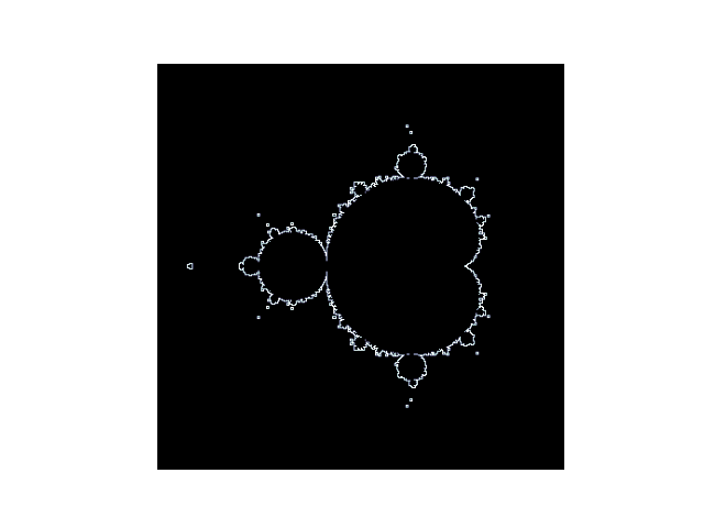
There are mutliple ways to get the edges of a shape using this method. We chose to use a kernel with only \(-1\) on its borders and a value \(k_5=8=-\sum_{i=1,\ i\neq 5}^9 k_i\). We also need to pad the image in order to get all the pixels in it, and not forget the borders. Let’s take a look at the result.

import chaoseverywhere as chaos
import numpy as np
import matplotlib.pyplot as plt
from scipy.signal import convolve2d

mandel = chaos.Mandelbrot_disp(-.5, 0, 1.5).mandelbrot()
kernel_edge_detect = np.array([[-1, -1, -1], [-1, 8, -1], [-1, -1, -1]])
pad_mandel = np.pad(mandel, ((1, 1), (1, 1)), "maximum")
bound = convolve2d(pad_mandel, kernel_edge_detect, mode='valid').astype(bool) * mandel

plt.imshow(bound, cmap='bone')
plt.axis('off')
plt.show()